Using the power of sound to figure out which Simpsons character is speaking
Update: you can find the next post in this series here.
In a previous post, I looked at transcripts of Simpsons episodes and tried to figure out which character was speaking which line.
This worked decently, but it wasn’t great. It gave us memorable scenes like this one:
Homer : D'oh! A deer! A female deer.
Marge : Son, you're okay!
Bart : Dad, I can't let you sell him. Stampy and I are friends. Ow!
Bart : Dad, how would you like to be sold to an ivory dealer?
Bart : Dad, you're sinking! Huh?
Marge : Get a rope, Bart. No, that's okay.
And this one:
Homer : I don't like this new director's cut.
Secondary : You're sskying a table? I'm not sskyin' it.
Tertiary : Ah. Is that my necktie you're wearing? Souvenir.
Bart : Mom, what if there's a really bad, crummy guy who's going to jail, but I know he's innocent.
Marge : Well, Bart, your Uncle Arthur used to have a saying ''Shoot 'em all, and let God sort 'em out.'' Unfortunately, one day he put his theory into practice.
And some not so memorable scenes:
Homer : Mmm, engineblock eggs.
Marge : Hey, it's morning, and Mom and Dad aren't home yet.
Tertiary : Hey. This isn't the Y.M.C.A.
Homer : Dispatch, this is Chief Wiggum back in pursuit of the rebelling women.
Homer : All right. Your current location? Oh. Uh, I'm a I'm on a road. Looks to be asphalt.
Trying to identify who is speaking only by looking at the text is a bit like trying to walk in a straight line with your eyes closed. There is a lot of information that you end up missing.
What if I told you that one of your friends asked me hey, how's it going?, and I asked you to figure out which friend. Even if you know someone for years and years, it won’t help you figure it out.
Enter the amazing sound wave. If I played you a sound clip of your friend saying the same phrase, you would almost instantly know who said it. Audio has a lot of information in this context that text cannot convey, and if we want to accurately identify our Simpsons characters, we need to use it.
As we progress, keep in mind that the code for this is available here, but this is the non-technical explanation. I will make a full technical post once I evaluate the various methods.
Quantifying sound
Sound is a tricky thing. It is pretty easy to look at a piece of text, and think of how a computer might process it, as computers work with text all the time. It’s a little different with sound, which can be very messy and indefinite.
Thankfully, we can exploit some properties of sound to ensure that it can be easily processed by computer. The first is that all sound is a wave.
What we see below is a plot of the beginning of the simpsons intro music:
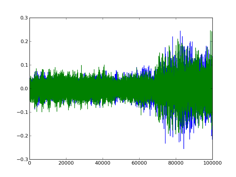 We can zoom in to actually see the lines:
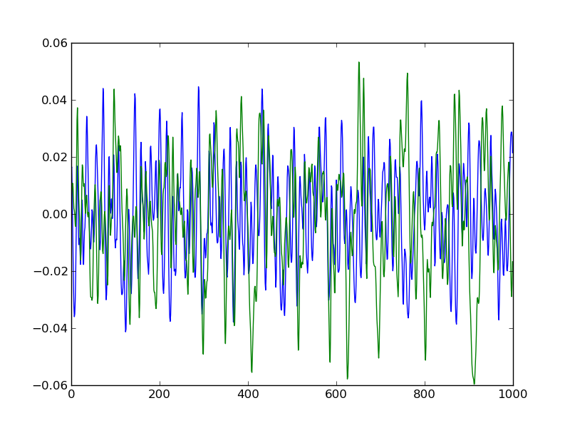 One of the lines is the right side audio, one of the lines is the left side audio. It doesn’t matter much which is which for our purposes, but let’s say that blue is left and green is right. Most audio now, including our Simpsons audio, is in stereo format, which means that there are 2 independent sources of sound. When you put on a pair of headphones, or listen to speakers, different sound plays on the left and right if you have stereo audio. Audio could also be in mono format, in which case we would only see one line. For our purposes, stereo means that we have two streams of sound to look at.
You can see that sound has some obvious tendencies. The sound wave is oscillating up and down, but the pattern is not always fixed, so one peak might be higher or lower than the one before it, and one local minimum might be lower or higher than the one before it. We can use these oscillations to differentiate between Simpsons characters.
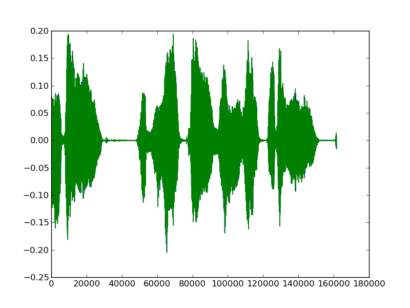
Here is Homer speaking the line Sure do! When you're 18,you're out the door!:
 And here is Lisa speaking the line
 No, Dad, you promised if Bart and I got "C" averages, we could go to Kamp Krusty.:
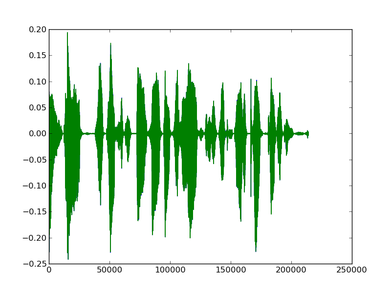 We can note distinct differences between the two. A lot of this is due to the different words being spoken, but we can hope that at least some of it is due to the unique voice of Lisa as compared to Homer.
How do we do this?
When we start, we have subtitle files, which look like this:
282
00:17:32,523 --> 00:17:35,651
I am so Krunchy the Clown!
[ Belches ]

283
00:17:35,760 --> 00:17:37,955
All right. That's it.

284
00:17:38,062 --> 00:17:40,326
I've been scorched by Krusty before.

285
00:17:40,431 --> 00:17:42,899
I got a rapid heartbeat
from those Krusty Brand vitamins.

286
00:17:43,000 --> 00:17:45,468
My Krusty calculator
didn't have a seven or an eight!
We also have the episodes from some of the Simpsons seasons (well, I do, at least).
We want to do two main things:
- Correlate the lines in the subtitles to the lines in the videos
- Make the video into a format that can be used for predictions
The first thing is relatively easy. This line 00:17:32,523 --> 00:17:35,651 is timing information, that tells us that Barney is pretending to be Krusty from 17 minutes and 32 seconds into the episode until 17 minutes and 35 seconds into the video. We can parse the subtitle file to get the whole line, when the line started in seconds, and when the line ended in seconds, for each of the lines in an episode.
Now, we just have the easy task of getting the audio out of the video and making and algorithm understand it. Right?
Working with audio
The first thing that we need to do is extract the audio tracks from our video files, which is easy with a tool like ffmpeg.
Once we convert the episodes to audio-only, we can read the audio files and process them.
Reading them in gives us what is an array:
Here, 2 is our number of audio channels (in this case, we have stereo audio, so a right and a left).
The length of the array (n) matches up with the length of our episode, and is determined by the sampling frequency of the sound. The sampling frequency determines how many times per second the sound wave was measured and recorded. The higher the sampling frequency, the bigger n would be for the same length of audio. For example, Season 4, Episode 12 (Marge vs. the Monorail) is 23 minutes and 5 seconds long. When we read in the episode, we get a array. The sampling frequency of this is 48000.
So, our audio array has the same length as the episode. We have timing information in seconds from our handy subtitle file, and we can match that up with the audio tracks to extract the lines that the characters are speaking.
Audio fingerprinting
We talked before about different voices having unique oscillations and features.
We can quantify these unique differences (features), and use them to “fingerprint” individual characters. These features are things such as how high on average the wave for a particular speaker is, how low on average the wave is, zero crossing rate, and cepstrum. We generate each of our features for each line of character audio that we have extracted.
Once we have these features, we can train a machine learning algorithm to predict who is speaking.
For the algorithm to work, we need to have labelled data, that is, we need subtitles that we have already identified a speaker for. I sacrificed 30 minutes of my life in the name of science to do this labelling for portions of a few episodes. This gives our algorithm the initial training to predict speakers.
In rough terms, the algorithm will:
- Read in our input features
- Correlate our training labels with the features in the labelled lines
- Create a model mapping features to labels
- Predict the labels for the unlabelled lines
Visualizing the audio
We can visualize our labelled lines and their predicted classifications in 2 dimensions with an SVM classification plot:
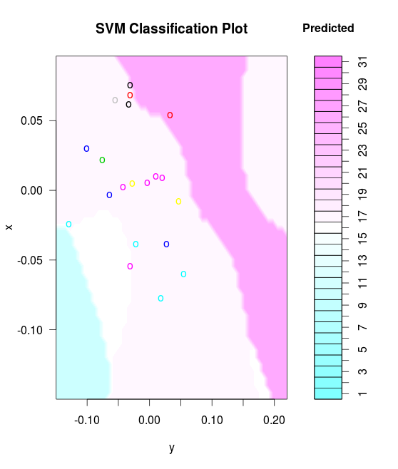 This shows up where the support vectors between the classes (labels) are, and where they fall.
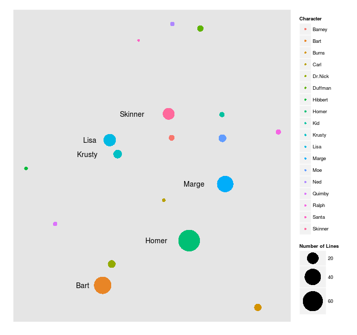
We can also take our audio features, and use them to visualize the characters in two dimensions. This first plot shows you how vocally dissimilar (or similar) the characters are in the small initial sample of text that I hand-labelled, which comes out to 313 lines across 5 episodes. The larger a dot is, the more lines that character had.
 Now, we can use the algorithm to finish labelling the remaining lines of those 5 episodes. This gives us 1544 lines, and a different plot:
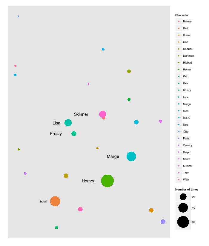 Update: And here is the plot for 192 episodes across 10 seasons. In this case, the size of the dot is log scaled.
 We can also directly look at the lines and compare accuracy. Label is the hand label, and predicted label is what the algorithm predicted:
                                                                          Line Label Predicted Label season episode
79 - "Yello." Homer Homer 1 1
80 - Marge, please.|- Who's this? Patty Patty 1 1
81 May I please speak to Marge? Patty Patty 1 1
82 - This is her sister, isn't it?|- Is Marge there? Homer Homer 1 1
83 - Who shall I say is calling?|- Marge, please. Homer Homer 1 1
84 It's your sister.|Oh! Homer Homer 1 1
85 - Hello.|- Hello, Marge. It's Patty. Patty Homer 1 1
86 Selma and I couldn't be more excited|about seeing our sister Christmas Eve. Patty Patty 1 1
87 Well, Homer and I are looking|forward to your visit too. Marge Marge 1 1
88 Somehow I doubt|that Homer is excited. Patty Patty 1 1
89 of all the men|you could've married, Patty Patty 1 1
We can define two simple error metrics to figure out how we are doing.
The first is adjacent correctness. So, if our result label occurs in a window +/- from the actual label, then we mark it as “adjacent correct.” This is because the subtitle timing information is not always perfect, and multiple characters can also speak in one subtitle line, making labelling difficult. So, line 85 above would be “adjacent correct” because Homer is speaking in line 84, meaning the predicted label (Homer) occured in the actual labels one line before.
We can define exact correct to mean that the result label and the actual label are the same.
The perils of error estimation
I had initially used cross validation to measure error. Cross validation involves randomly splitting up a dataset and using some sections to predict other sections. I realized after the fact that this made the correct rate way too high. Using cross validation, for example, allows the algorithm to use some of the lines from Season 1, Episode 1, which I hand labelled the beginning of, to predict the rest.
Our “adjacent correct” rate with cross validation is 291/313, or 93%, and our exact correct rate is 275/313, or 87.8%.
Instead of using cross validation, we can do something I call “sequential validation”, where we treat each episode separately, and predict each episode with data from all other episodes.
When we do this, our adjacent correct rate is 142/313, or 45%, and our exact correct rate is 84/313, or 27%. With only 313 labelled training lines, this is a pretty good result.
What can we do with this?
I originally wanted to do some linguistic analysis on the Simpsons episodes, and we are getting to that point (although I did say that last time, playing with sound is just too cool to pass up).
We could make some improvements to this:
- Combine the NLP based approach from last time with the audio based approach from this time.
- Hand label more training lines (this will increase accuracy a lot).
- Exploit the data to “auto-label”. For instance, some lines say [Burns] or [Marge] when the character isn’t on screen.
- Correlate the labelled data used in the last post with the subtitles used here to generate labelled data.
- Generate more/better audio features.
Ultimately, the general approach to improving an algorithm is more data, more approaches, more features, and we cover those bases here.
Once my machine gets through labelling all of the lines (processing the audio streams takes a long time! Update: It finished, see the plot above.), I will look into refining the method a bit, and then do some linguistic analysis (ever wanted to know how much the characters like each other?).
Would be happy to hear any comments/suggestions. And after writing this post, I need a beer, so here’s to alcohol,the cause of, and solution to, all of life’s problems.
