Linear Regression from the Ground Up

Linear regression is a very basic technique that we use a lot in machine learning. In a lot of cases (and I have been guilty of this), we just use it without much thought as to how the internals actually work.

In a 2-D coordinate system, we can plot observations (such as, a child’s age is 1), and associated dependent variables (ie, the child has 1 friend) on an x/y axis, like the one below: 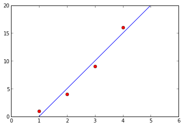linear regression In the above system, we have plotted several observation and dependent variable pairs [1,1], [2,4], [3,9], [4,16]. We have also added in a line. This line allows us to predict the dependent variables for future observations (when the child is 5, according to our line, they will have 20 friends). The line is defined by an equation $y=bx+a$ where b is the slope of the line, and a is the y-intercept. In the simplest form of linear regression, we can figure out b and a to find the line. In more complex forms, such as $y=b_{1}x_{1} + b_{2}x_{2}+a$ , we can predict y using multiple features.

Today, I’m going to shed some light on the internals to linear regression, and do some comparisons of various approaches in Python. If you have not read my earlier post on matrix inversion, I highly recommend it.

Setup

As you can see from the line and points above, the point of linear regression is to minimize the sum of squared errors between the actual y value and the predicted y value.

We can express the various pairs in matrix form using the equation $y=bX + e$ where X is the matrix of X observations, y is the vector of dependent values, b is the vector of coefficients, and e is a vector of errors (which we want to minimize).

\begin{bmatrix} 1 \\ 4 \\ 9 \\ 16 \end{bmatrix}= \begin{bmatrix} 1 & 1 \\ 1 & 2 \\ 1 & 3 \\ 1 & 4 \end{bmatrix} \begin{bmatrix} b_{0} \\ b_{1} \end{bmatrix} + \begin{bmatrix} e_{1} \\ e_{2} \\ e_{3} \\ e_{4} \end{bmatrix}

We add in an extra column on the left of the X matrix to create the intercept, which is $b_{0}$ . We can multiply out the matrices to get:

\begin{bmatrix} 1 \\ 4 \\ 9 \\ 16 \end{bmatrix}= \begin{bmatrix} 1b_{0} + 1b_{1} + e_{1} \\ 1b_{0} + 2b_{1} + e_{2} \\ 1b_{0} + 3b_{1}+ e_{3} \\ 1b_{0} + 4b_{1}+ e_{4} \end{bmatrix}

So, we want to solve for $b_{0}$ and $b_{1}$ in a way that minimizes the error.

Minimizing Error

We can model the sum of squared errors of the above system as:

\begin{bmatrix} e_{1} & e_{2} & e_{3} & e_{4} \end{bmatrix} \begin{bmatrix} e_{1} \\ e_{2} \\ e_{3} \\ e_{4} \\ \end{bmatrix}

This will simplify to $$ e1^2 + e2^2 + e3^2 + e4^2 $$.

Our first matrix is the transpose of the second matrix. We can denote the transpose as $E^{T}$ , and the original as E.

Error just refers to predicted values minus actual values. In this case, our actual values are in the y vector, and our predicted values are bX.

So, our squared error is $E^{T}E=(Y-Xb)^{T}(Y-Xb)$ .

Setting error to zero (we want to minimize it) and taking the derivative with respect to b gives us $-2X^{T}(y-Xb)=0$ . We can then multiply this out to get $X^{T}y=X^{T}Xb$ , and finally $b=(X^{T}X)^{-1}(X^{T}y)$ .

So, this is starting to look easier. To get our coefficients, we just solve:

b=(X^{T}X)^{-1}(X^{T}y)

Implementation - Matrix class

All the implementation code is available in the algorithms repository.

In order to implement the algorithm, we first need to define a basic class for a matrix. Here is some excerpted code.

class Matrix(object):
    """
    Represent a matrix and allow for basic matrix operations to be done.
    """
    def __init__(self, X):
        """
        X - a list of lists, ie [[1],[1]]
        """
        #Validate that the input is ok
        self.validate(X)
        self.X = X

We can then write class methods to perform the operations that we need (inversion, transposition, and multiplication). Inversion was covered in a previous post, so our code is short:

def invert(self):
    """
    Invert the matrix in place.
    """
    self.X = invert(self.X)
    return self

Transposition:

def transpose(self):
    """
    Transpose the matrix in place.
    """
    trans = []
    for j in xrange(0,self.cols):
        row = []
        for i in xrange(0,self.rows):
            row.append(self.X[i][j])
        trans.append(row)
    self.X = trans
    return self

Multiplication can be added by overriding __mul__. See the magic methods guide for information.

def __mul__(self, Z):
    """
    Left hand multiplication, ie matrix * other_matrix
    """
    assert(isinstance(Z, Matrix))

    assert Z.rows==self.cols

    product = []
    for i in xrange(0,self.rows):
        row = []
        for j in xrange(0,Z.cols):
            row.append(row_multiply(self.X[i], [Z[m][j] for m in xrange(0,Z.rows)]))
        product.append(row)
    return Matrix(product)

__rmul__ can also be overridden for right hand multiplication (and is in the algorithms repository).

Implementation – Multivariate Regression

Then, we can implement the regression.

class LinregCustom(Algorithm):
    """
    Solves for multivariate linear regression
    """
    def train(self, X, y):
        """
        X - input list of lists
        y - input column vector in list form, ie [[1],[2]]
        """
        assert len(y) == len(X)
        X_int = self.append_intercept(X)
        coefs = ((Matrix(X_int) * Matrix(X_int).transpose()).invert())
        coefs = (Matrix(X_int).transpose()) * coefs
        coefs = coefs * Matrix(y)
        self.coefs = coefs

    def predict(self,Z):
        """
        Z - input list of lists
        """
        Z = self.append_intercept(Z)
        return Matrix(Z) * self.coefs

    def append_intercept(self, X):
        """
        Adds the intercept term to the first row of a matrix
        """
        X = deepcopy(X)

        #Append this to calculate the intercept term properly
        for i in xrange(0,len(X)):
            X[i] = [1] + X[i]
        return X

We can try this:

lr = LinregCustom()
lr.train([[1,2,1],[2,3,2],[3,1,2],[4,2,1]], [[1],[4],[9],[16]])
print(lr.predict([[1,2,1],[2,3,2],[3,1,2],[4,2,1]]))

[[0.9999999999999991], [3.9999999999999982], [8.999999999999993], [15.999999999999996]]

Although the numbers may not be exact, you should get similar output to this. This essentially reconstructs our original inputs.

Implementation – Univariate Regression

We can fall back on a univariate linear regression formula:

class LinregNonMatrix(Algorithm):
    """
    Solve linear regression with a single variable
    """
    def train(self, x, y):
        """
        x - a list of x values
        y - a list of y values
        """
        x_mean = mean(x)
        y_mean = mean(y)
        x_dev = sum([abs(i-x_mean) for i in x])
        y_dev = sum([abs(i-y_mean) for i in y])

        self.slope = (x_dev*y_dev)/(x_dev*x_dev)
        self.intercept = y_mean - (self.slope*x_mean)

    def predict(self, z):
        """
        z - a list of x values to predict on
        returns - computed y values for the input vector
        """
        return [i*self.slope + self.intercept for i in z]

lr = LinregNonMatrix()
lr.train([1,2,3,4], [1,4,9,16])
lr.predict([1,2,3,4])

[0.0, 5.0, 10.0, 15.0]

This will not pick up the clear nonlinearity in the input series, which is $Y=X^{2}$ .

Implementation – Regression with Numpy

We can also use Numpy to solve a linear regression for us.

class LinregNumpy(Algorithm):
    """
    Use numpy to solve a multivariate linear regression
    """
    def train(self,X,y):
        """
        X - input list of lists
        y - input column vector in list form, ie [[1],[2]]
        """
        from numpy import array,linalg, ones,vstack
        assert len(y) == len(X)
        X = vstack([array(X).T,ones(len(X))]).T
        self.coefs = linalg.lstsq(X,y)[0]
        self.coefs = self.coefs.reshape(self.coefs.shape[0],-1)

    def predict(self,Z):
        """
        Z - input list of lists
        """
        from numpy import array, ones,vstack
        Z = vstack([array(Z).T,ones(len(Z))]).T
        return Z.dot(self.coefs)

We can reproduce the same predictions that we got with our multivariate regression.

lr = LinregNumpy()
lr.train([[1,2,1],[2,3,2],[3,1,2],[4,2,1]], [[1],[4],[9],[16]])
print(lr.predict([[1,2,1],[2,100,2],[3,2,2],[4,2,1]]))

[[ 1.]
 [ 4.]
 [ 9.]
 [ 16.]]